Urban heat is a major issue in Dubai. By identifying where heat stress is worst and where interventions would help the most people, planners can make better decisions about:
Where to plant trees
Where to add shade structures
Which streets to prioritize for pedestrian improvements
2. Data Sources
2.1 Mapillary Street View Images
Property
Value
Source
Mapillary (crowdsourced street imagery)
Images downloaded
11,651
Coverage
Al Karama district boundary
Cost
Free (API access)
Tool used
ZenSVI Python library
# How we downloaded images
from zensvi.download import MLYDownloader
mly = MLYDownloader(log_path="logs")
mly.download_svi(
dir_output="data/mapillary_svi",
input_shp="data/al_karama.geojson",
lat=None, lon=None,
id_columns=None
)
Google Earth Engine (GEE): We used GEE to access and process satellite data. It's free for research/academic use. You need to register at earthengine.google.com.
GEE also hosts the JRC Global Human Settlement Layer (GHSL), which provides satellite-derived building height data globally. We used the GHSL Built-C (10m categorical height classes) and Built-H (100m continuous heights) datasets to fill in the majority of building heights that were missing from OpenStreetMap (see Section 5).
Seasonal satellite analysis: Both Landsat and Sentinel-2 are filtered per season — summer 2025 (Jun–Sep) and winter 2025/26 (Dec–Feb) — so that all satellite indices reflect the same time window. Filtering by season (vs. a full-year composite) is important because vegetation indices like NDVI are season-dependent, and comparing summer vs. winter reveals how the urban heat island effect shifts with solar geometry. The viewers include a season dropdown to switch between summer and winter data.
pois_cache.json — avoids repeat API calls on re-run
Noise filtering: 18 OSM types are excluded as "urban furniture" that would clutter the map: bench, waste_basket, parking, shelter, bollard, fire_hydrant, street_lamp, etc. This reduces the raw 1,419 elements to 1,290 meaningful PoIs.
3. Street View Analysis
3.1 Green View Index (GVI)
What it measures: The percentage of green pixels (vegetation) visible in a street view image.
GVI = (Green pixels in image) / (Total pixels in image) × 100%
How it's calculated:
Take a street view image
Convert to a color space that separates green vegetation
Use a vegetation index formula to identify green pixels
Count the percentage of green pixels
Al Karama Result: Mean GVI = 3.55%
This is very low - most streets have minimal visible vegetation.
View GVI on 2D Viewer →
3.2 Sky View Factor (SVF)
What it measures: The percentage of sky visible from a point on the street. Lower SVF = more shading from buildings/trees.
SVF = (Sky pixels in image) / (Total pixels in upper hemisphere) × 100%
Interpretation:
SVF = 100%: Open area, no obstructions (full sun exposure)
SVF = 50%: Half the sky blocked (moderate shading)
SVF = 20%: Narrow street canyon (good shading)
Al Karama Result: Mean SVF = 31.4%
Moderate sky exposure - some shading from buildings but not dense urban canyon.
View SVF on 2D Viewer →
What it measures: The temperature of the ground/surface as seen from space.
Important: LST is NOT air temperature. It measures how hot surfaces (roads, buildings, sand) are. LST is typically higher than air temperature during the day.
How it's calculated from Landsat:
LST = Brightness Temperature / (1 + (λ × BT / ρ) × ln(ε))
Where:
λ = wavelength of thermal band (10.8 μm)
BT = brightness temperature from satellite
ρ = h × c / σ (Planck's constant × speed of light / Boltzmann)
ε = surface emissivity (assumed 0.95 for urban areas)
Al Karama Result:
Mean LST = 48.3°C (summer)
Range: 36°C to 55°C
The 18°C variation shows some areas are significantly cooler (likely parks/vegetation).
View LST on 2D Viewer →
4.2 NDVI (Normalized Difference Vegetation Index)
What it measures: Vegetation health/density from satellite perspective.
NDVI = (NIR - Red) / (NIR + Red)
Where:
NIR = Near-infrared reflectance (Sentinel-2 Band 8)
Red = Red reflectance (Sentinel-2 Band 4)
Interpretation:
NDVI Value
Meaning
-1.0 to 0
Water, bare soil, buildings
0 to 0.2
Sparse vegetation, dry grass
0.2 to 0.4
Moderate vegetation
0.4 to 0.6
Dense vegetation
0.6 to 1.0
Very dense, healthy vegetation
Al Karama Result: Mean NDVI = 0.096
Very low - mostly built-up with sparse vegetation.
View NDVI on 2D Viewer →
What it does: Downscales coarse Landsat thermal data (30m) to match Sentinel-2 resolution (10m) using the correlation between temperature and vegetation.
Why it's needed: Landsat thermal bands have 100m native resolution (resampled to 30m). For detailed urban analysis, we want finer resolution to see temperature variations at street level.
Method: Linear regression of LST vs NDVI at 30m → Apply model to 10m NDVI
1. Sample both LST (30m) and NDVI (10m aggregated to 30m) at random points
2. Fit regression: LST = a + b × NDVI
3. Apply to 10m NDVI: LST_10m = a + b × NDVI_10m
4. Add residuals from nearest 30m pixel for local calibration
Al Karama Result:
Regression: LST = 49.02 + (-3.66 × NDVI)
R² = 0.045 (weak correlation)
RMSE = 0.32°C (difference between 30m and 10m)
Note: Weak R² is expected in urban areas where impervious surfaces dominate. The method works better in areas with more vegetation variation.
5. Building Height Enhancement (GEE)
5.1 The Problem
OpenStreetMap provides building footprints for Al Karama (3,243 buildings), but only 78 buildings (2.4%) have real height data. The remaining 3,165 buildings default to 9m (assumed 3 floors), which produces an unrealistic 3D model where most buildings appear the same height.
Goal: Use freely available global datasets from Google Earth Engine to estimate building heights for the 97.6% of buildings missing real data.
5.2 Datasets Evaluated
We tested multiple GEE datasets for coverage over Dubai/Al Karama:
Dataset
Resolution
Coverage
What it provides
Open Buildings 2.5D Temporal
~2.5m
Not available (0 images)
Would have had individual building heights
GHSL Built-C
10m
84,182 pixels
Height classes (categorical)
GHSL Built-H
100m
883 pixels
Continuous heights (meters)
nDSM (ALOS-SRTM)
30m
10,416 pixels
Surface model difference
5.3 GHSL Built-C (10m) - Height Classes
Source: JRC Global Human Settlement Layer (GHSL), 2018 epoch
Collection:JRC/GHSL/P2023A/GHS_BUILT_C/2018
This dataset classifies built-up areas into height bands at 10m resolution. Each pixel encodes both building type (residential, non-residential, mixed) and height class:
Height Class
Range
Midpoint Used
1
≤3m
3.0m
2
3-6m
4.5m
3
6-15m
10.5m
4
15-30m
22.5m
5
>30m
45.0m
Method: For each OSM building polygon, we used reduceRegions with a mode reducer to extract the dominant height class within the footprint, then converted to the midpoint height.
# Extract height class per building polygon
image = ee.Image("JRC/GHSL/P2023A/GHS_BUILT_C/2018")
band = image.select('built_characteristics')
reduced = band.reduceRegions(
collection=building_polygons,
reducer=ee.Reducer.mode(),
scale=10,
)
# Convert class to height: height_band = class_value % 10
# Then map to midpoint heights
5.4 GHSL Built-H (100m) - Continuous Heights
Collection:JRC/GHSL/P2023A/GHS_BUILT_H/2018
Provides continuous building height estimates in meters at 100m resolution. Less spatial detail but gives actual meter values rather than classes.
Method:reduceRegions with mean reducer per building polygon.
Limitation: GHSL Built-H caps at ~40m for this area (mean 13.5m). Al Karama has buildings taller than 40m, so GHSL may underestimate the tallest buildings. OSM real heights (up to 230m) are preserved where available.
5.5 nDSM: Normalized Digital Surface Model (30m)
What it is: The difference between a Digital Surface Model (DSM, which includes buildings/trees) and a Digital Elevation Model (DEM, bare ground only).
Positive nDSM values indicate above-ground structures (buildings, trees). However, this approach is noisy because the two datasets were acquired years apart (2000 vs 2006-2011), and both have their own measurement uncertainties.
Limitation: The temporal mismatch between SRTM (2000) and ALOS (2006-2011) means buildings constructed between these dates will appear in the nDSM, but pre-existing terrain changes or demolitions can produce artifacts. We applied a threshold of >2m to filter out noise.
5.6 Priority Merge System
We merged heights from all sources using a priority system that preserves the most reliable data:
Priority
Source
Resolution
Rationale
1 (highest)
OSM real height (≠9m)
Individual
Surveyed or mapped by contributors
2
GHSL Built-C
10m
Best spatial resolution, height classes
3
GHSL Built-H
100m
Continuous values but coarser
4
nDSM
30m
Noisy but independent measurement
5 (lowest)
Default
n/a
Keep 9m assumption
5.7 Results
Coverage improved from 2.4% to 99.5%:
Source
Buildings
Percentage
OSM real height
78
2.4%
GHSL Built-C (10m)
3,055
94.2%
GHSL Built-H (100m)
80
2.5%
nDSM (30m)
14
0.4%
Default (9m)
16
0.5%
Total with data
3,227
99.5%
GHSL Built-C dominated because its 10m resolution matches well with building footprint sizes, and it had near-complete coverage of the study area. The 3D visualization now includes a "Color by Source" toggle to show which dataset provided each building's height.
Height distribution by source:
OSM real: 6-230m (median 36m) - includes known tall buildings
GHSL Built-C: 3-45m (median 10.5m) - 5 height classes
GHSL Built-H: 2.5-33.7m (median 10.3m) - continuous
nDSM: 2.7-10.8m (median 4.0m) - low-rise buildings only
6. Combined Analysis
6.1 Heat Mitigation Priority
Goal: Identify locations where interventions (tree planting, shade) would have the most impact.
Method: Combine multiple factors into a priority score:
Network analysis treats streets as a graph (nodes = intersections, edges = street segments) to understand which streets are most important for movement.
7.2 Betweenness Centrality
What it measures: How often a street lies on the shortest path between other locations.
Betweenness(v) = Σ (σst(v) / σst)
Where:
σst = total number of shortest paths from node s to node t
σst(v) = number of those paths that pass through v
Interpretation: High betweenness = many people pass through this street to get from A to B. These are main corridors.
We combined centrality with comfort to find streets where improvements help the most people:
Intervention Priority = Centrality × (1 - Comfort)
High priority = busy street that is uncomfortable
Result: 51 streets identified as high priority - heavily used but uncomfortable.
7.5 Edge Effects
Important caveat: Centrality calculations are affected by study area boundaries. Streets at the edge appear less important because paths can't continue beyond our boundary. We addressed this by expanding the analysis area (+500m buffer) and then clipping results back to Al Karama.
8. Cluster Analysis
8.1 K-Means Clustering
Goal: Group locations into distinct "urban climate zones" based on their characteristics.
Method:
Select features: GVI, SVF, LST, NDVI
Standardize features (z-scores) so they're comparable
Quantify how much shade buildings and tree canopies cast on streets during peak summer, and identify which streets are most exposed to direct sun. This extends the building height data (Section 5) and integrates tree canopy data from the Meta 1m Global Canopy Height Map.
Method: Implemented the NOAA solar position spreadsheet algorithm using pure numpy/math (no external solar libraries). The algorithm computes solar altitude and azimuth from Julian Day, solar declination, hour angle, and observer coordinates.
Julian Day → Solar Declination → Hour Angle → Altitude & Azimuth
Analysis dates: July 15 (peak summer) and January 15 (mid-winter), 7 time slots from 6 AM to 6 PM.
Summer (July 15):
Local Time
Altitude
Azimuth
Shadow Length Factor
06:00
3.8°
68.0° (ENE)
15.23× height
08:00
29.7°
78.6° (E)
1.75×
10:00
56.7°
88.9° (E)
0.66×
12:00
83.2°
122.4° (SE)
0.12× (near overhead)
14:00
67.9°
265.0° (W)
0.41×
16:00
40.8°
277.3° (W)
1.16×
18:00
14.3°
287.3° (WNW)
3.93×
Winter (January 15):
Local Time
Altitude
Azimuth
Shadow Length Factor
06:00
−14.9°
106.7° (ESE)
Below horizon
08:00
10.1°
119.3° (ESE)
5.61× height
10:00
31.3°
138.9° (SE)
1.64×
12:00
43.2°
171.0° (S)
1.07×
14:00
38.6°
207.7° (SSW)
1.25×
16:00
20.8°
232.8° (SW)
2.63×
18:00
−2.8°
248.0° (WSW)
Below horizon
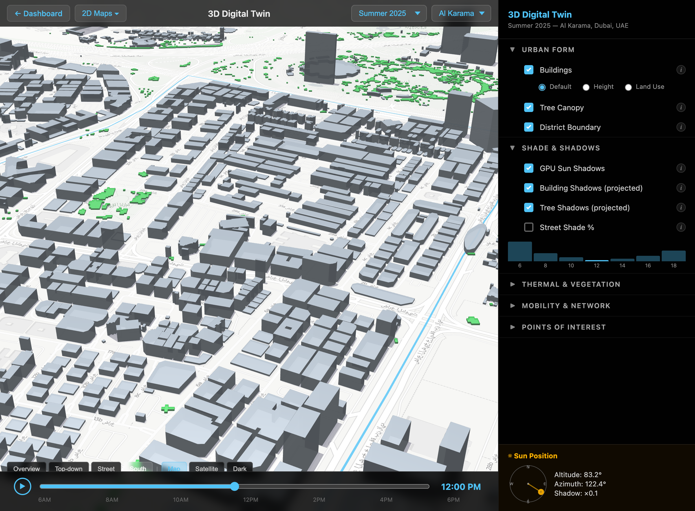
Key insight — summer: At noon in July, the sun is nearly overhead (83.2° altitude) so shadows are minimal (0.12× building height). Early morning and late afternoon produce extremely long shadows — at 6 AM the sun is only 3.8° above the horizon, casting shadows over 15× building height.
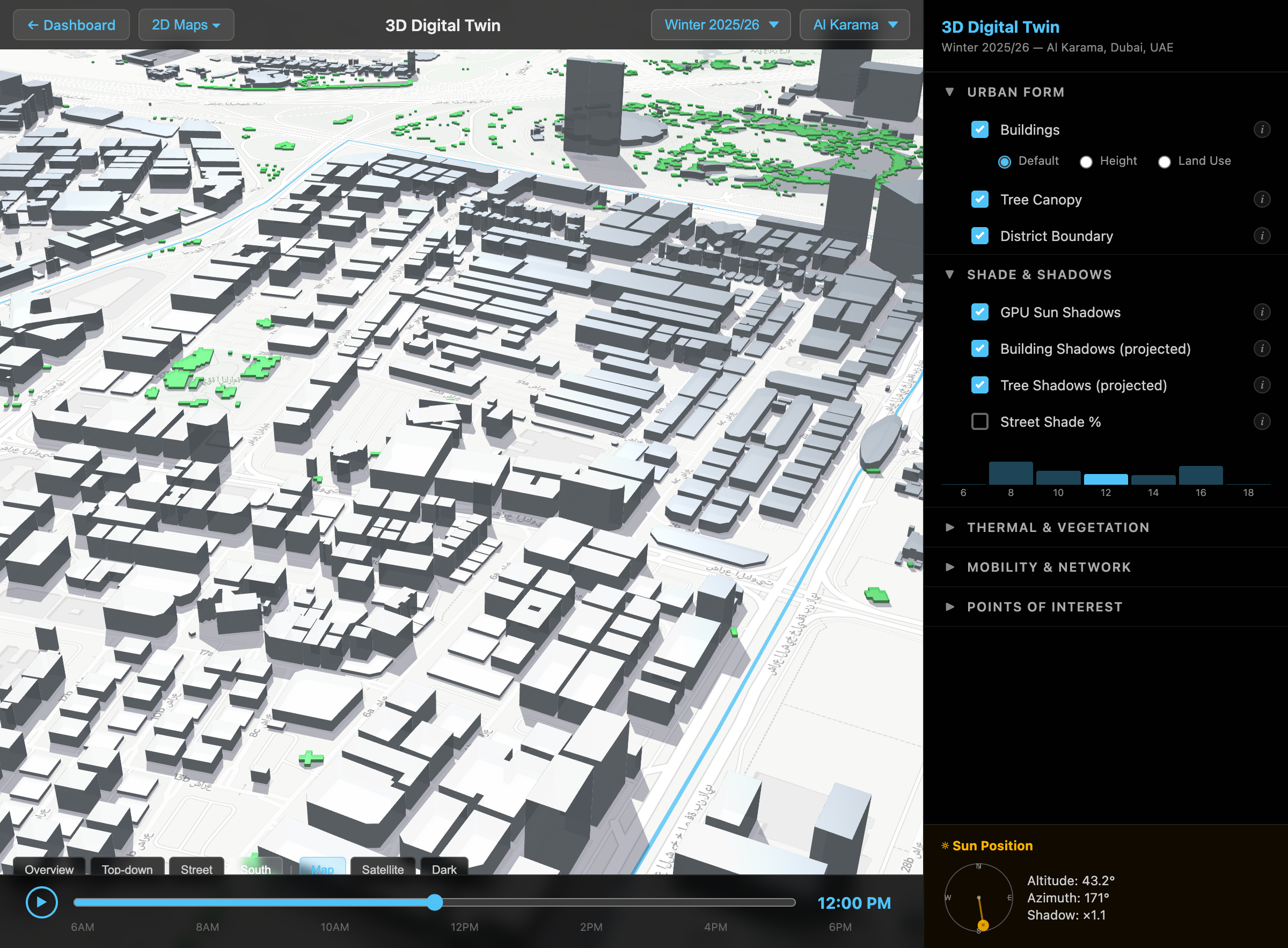
Key insight — winter: In January, the sun never climbs above 43.2° (at noon), meaning shadows are always at least 1× building height even at midday. At 6 AM and 6 PM the sun is below the horizon entirely — no direct sun exposure. The sun's arc shifts south, with azimuth ranging from ESE (119°) to SW (233°) instead of summer's nearly east–west path (68°–287°). This produces fundamentally different shadow patterns that favour north-facing streets.
9.3 Shadow Projection Method
For each building and tree canopy polygon at each time:
Shadow sources include 3,243 buildings and 1,033 tree canopy polygons, producing ~30,000 individual shadow projections across 7 time slots.
9.4 Tree Canopy Integration
Data source: Meta 1m Global Canopy Height Map, accessed via Google Earth Engine. The canopy data was processed in three stages:
Canopy polygon extraction: The raster canopy height image was thresholded (>2m) and converted to 1,033 vector polygons representing tree canopy areas.
Height sampling: 183 sample points with canopy height values were extracted from the raster.
IDW height interpolation: Each polygon centroid was assigned a height using Inverse Distance Weighting (IDW) interpolation from the 3 nearest sample points (within 500m). Polygons with no nearby samples received the median height (3.0m).
height_polygon = Σ(wi × hi) / Σ(wi), where wi = 1 / di²
Canopy Metric
Value
Total canopy polygons
1,033
Height range
1.0 – 11.9 m
Mean height
3.2 m
Median height
2.7 m
Sample points used for IDW
183
9.5 Street Shade Calculation
Method: For each time slot, union all building and tree canopy shadows using a chunked spatial approach (200m grid tiles), then calculate the fraction of each street segment that falls within shadow.
shade_fraction = shaded_length / total_length
Daily average shade is computed across all 7 time slots. Performance is managed via spatial indexing (STRtree) and chunked union operations.
9.6 Results
Time
Avg Shade
Well-shaded (≥50%)
Exposed (<20%)
06:00 AM
93.8%
5,339 / 5,656
155
08:00 AM
39.4%
2,250 / 5,656
1,842
10:00 AM
19.9%
1,106 / 5,656
3,249
12:00 PM
5.9%
288 / 5,656
5,052
02:00 PM
13.2%
722 / 5,656
3,907
04:00 PM
26.6%
1,511 / 5,656
2,570
06:00 PM
51.6%
3,015 / 5,656
1,309
Daily summary (buildings + trees combined):
• Average shade coverage across 7 time slots: 35.8%
• Well-shaded streets (≥50% daily average): 1,208 / 5,656 (21%)
• Exposed streets (<20% daily average): 1,639 / 5,656 (29%)
• Most shade at 6 AM (93.8%) and 6 PM (51.6%) — long shadows from low sun angle
• Least shade at noon (5.9%) — sun nearly overhead at 83°
Key outputs:
• Shadow polygons for each of the 7 time slots (GeoJSON) — separate building and tree shadow layers
• Shade percentage per street per hour (CSV, 5,656 streets × 7 hours)
• Interactive 2D map with time slider, building shadow toggle, and tree shadow toggle
• Interactive 3D map with extruded buildings (gray) and tree canopy (green), projected shadow overlays, and GPU-rendered sun shadows
• Streets colored by shade coverage (red=exposed, green=shaded)
9.7 Visualisation
Two interactive HTML maps are provided:
2D viewer (viewer_2d.html): Leaflet map with togglable analysis layers including street centrality, pedestrian comfort, heat priority, combined SVI, satellite grid, clusters, and green access. Exportable as SVG and PDF.
3D Digital Twin (viewer.html): deck.gl map with extruded buildings, green tree canopy polygons, and 1,290 Overpass API Points of Interest shown as emoji icons (🍛🛍️🏨 etc.) with category filter pills. Features both pre-computed projected shadow overlays (building + tree, toggleable) and GPU-rendered sun shadows via deck.gl _SunLight. Time slider controls shade simulation from 6 AM to 6 PM. Tooltips show building height, tree height, PoI name/category, and per-street shade percentage.
9.8 Points of Interest (Overpass API)
Objective: Overlay a rich, categorized layer of Points of Interest on the 3D shade map so users can see which amenities (restaurants, shops, clinics, schools, etc.) exist in relation to shade coverage.
Data Source
PoIs are fetched from the Overpass API, the public query interface for OpenStreetMap. A single bounding-box query retrieves all nodes and ways tagged with amenity, shop, tourism, office, leisure, or healthcare within the Al Karama study area.
Categorize: Map ~50 OSM tag values to 8 categories using a lookup table; unmapped shop=* tags default to "shopping"; all others default to "services"
Label: Use the name tag if available; otherwise title-case the OSM type (e.g., fast_food → "Fast Food")
Cache: Results saved to pois_cache.json (146 KB); subsequent runs load from cache without an API call
Result: 1,290 PoIs across 8 categories:
Category
Emoji
Count
Example OSM tags
Shopping
🛍️
462
supermarket, clothes, electronics, jewelry
Services
🏦
362
bank, atm, laundry, hairdresser, police
Food
🍛
282
restaurant, cafe, fast_food, bakery
Hotel
🏨
64
hotel, guest_house, apartment
Leisure
⚽
51
park, sports_centre, cinema, playground
Health
⚕️
48
pharmacy, clinic, hospital, dentist
Religious
🕌
12
place_of_worship
Education
🎓
9
school, kindergarten, driving_school
Visualisation
PoIs are rendered on the 3D map as emoji icons using deck.gl's IconLayer. Each category emoji is pre-rendered onto a 64×64 HTML canvas and converted to a PNG data URL at page load, which the IconLayer displays as a full-color bitmap texture.
Collision filtering: deck.gl's CollisionFilterExtension automatically hides overlapping icons, keeping the display clean at any zoom level
Text labels: PoI names appear (via TextLayer) only when zoomed past level 18, also with collision filtering
Category filter pills: 8 toggle pills in the control panel let users show/hide individual categories; All/None buttons for bulk control
Depth-test disabled: Icons render on top of extruded 3D buildings (parameters: { depthTest: false })
Design decision — emoji over colored dots: Initial implementation used colored circles, but 8 categories produced too many similar colors (e.g., orange food vs amber education; green leisure vs green tree canopy). Emoji icons (🍛 🛍️ 🏨 etc.) are instantly distinguishable without relying on color differentiation.
9.9 Caveats
1. Flat terrain assumed: No elevation model used — all buildings and trees assumed on same ground plane.
2. Trees modeled as solid polygons: Real tree canopies are porous — light filters through leaves. Our model treats each canopy polygon as a solid shadow caster, overestimating tree shade somewhat.
3. Canopy heights via IDW interpolation: Only 183 sample points were available for 1,033 polygons. Heights were interpolated using IDW (k=3), introducing spatial smoothing. The 1m resolution of the source raster is reduced.
4. Quantized building heights: GHSL height classes produce discrete height values, leading to quantized shadow lengths.
5. No diffusion: Shadow boundaries are binary (shaded/not shaded) — no partial shade or penumbra modeled.
10. Seasonal & Temporal Comparison
10.1 Why Compare Seasons?
Dubai experiences extreme heat in summer but mild, pleasant winters. Comparing the two seasons reveals how solar geometry, temperature, and vegetation change — and whether shade infrastructure designed for summer also benefits winter pedestrians. The analysis pipeline now supports a --season flag, and both the 3D and 2D viewers include a season dropdown to switch between datasets.
In addition to comparing seasons within a single year, we now include Summer 2020 and Winter 2020/21 data, enabling a 5-year temporal comparison to observe how urban heat, vegetation, and built-up indices have changed over time. The viewer dropdown presents all four seasons: Summer 2020, Winter 2020/21, Summer 2025, and Winter 2025/26.
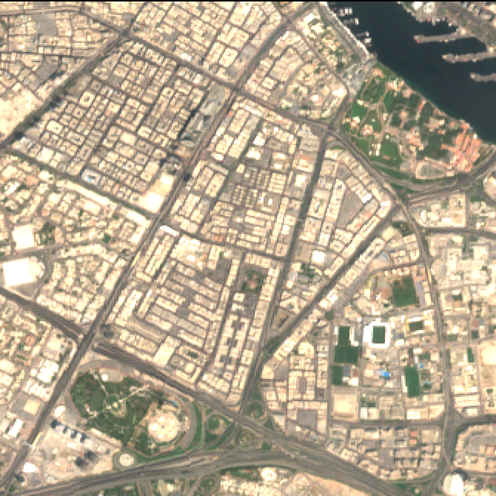
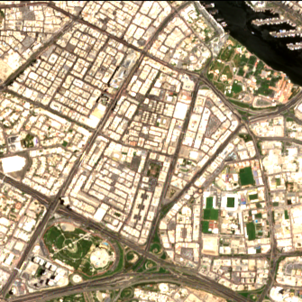
The Sentinel-2 true-colour images below show the same area (Al Karama, 10m resolution) five years apart. Each is the single clearest scene (lowest cloud cover) from the respective summer window. Click to enlarge.
The most striking difference between seasons is the sun's path across the sky:
Metric
Summer (Jul 15)
Winter (Jan 15)
Difference
Peak solar altitude (noon)
83.2°
43.2°
−40.0°
Noon shadow factor
0.12×
1.07×
~9× longer shadows
Sunrise/sunset (local)
~5:30 AM / 7:10 PM
~7:00 AM / 5:40 PM
~2.5 h shorter day
Usable analysis hours (sun > 0°)
7 (6 AM–6 PM)
5 (8 AM–4 PM)
−2 hours
Sun azimuth range
68°–287° (E–WNW)
119°–233° (ESE–SW)
Narrower, shifted south
Key implication: In summer, the sun passes nearly overhead, so only tall buildings cast meaningful noon shadows. In winter, even a 10m building casts a 10.7m shadow at noon. This means winter pedestrians benefit significantly more from existing building shade, especially on streets running east–west with buildings on the south side.
10.3 Shadow Coverage
The shadow projection analysis (Section 9) was run for both seasons. The lower winter sun produces dramatically more shade at midday, while summer's longer daylight hours produce shade at dawn and dusk when the winter sun is below the horizon:
Time
Summer Shade
Winter Shade
Change
06:00 AM
93.8%
0.0% (sun below horizon)
—
08:00 AM
39.4%
60.3%
+20.9 pp
10:00 AM
19.9%
35.6%
+15.7 pp
12:00 PM
5.9%
27.9%
+22.0 pp
02:00 PM
13.2%
25.2%
+12.0 pp
04:00 PM
26.6%
48.6%
+22.0 pp
06:00 PM
51.6%
0.0% (sun below horizon)
—
Key finding: Winter noon shade (27.9%) is nearly 5× the summer noon shade (5.9%). At the most critical midday hours (10 AM–2 PM), winter shade coverage averages 29.6% versus summer's 13.0%. This confirms that existing building geometry provides substantial passive shade in winter, while summer remains the season of greatest pedestrian heat stress.
10.4 Satellite Metric Differences
The satellite analysis was run for both seasons using Landsat 8/9 and Sentinel-2 data. The table below shows measured values (not projections):
Metric
Summer 2025
Winter 2025/26
Difference
LST mean
48.3°C
27.1°C
−21.2°C
LST range
35.9–54.8°C
21.4–33.0°C
~15°C lower across board
NDVI mean
0.096
0.114
+0.018 (slightly greener)
NDVI range
−0.14 to 0.78
−0.27 to 0.88
Wider range in winter
NDBI mean
0.033
0.010
−0.023
What this means for pedestrians:
Summer: Extreme heat (48.3°C surface, peak 54.8°C) + minimal shade at peak hours (5.9% at noon) = severe heat stress. Shade interventions are critical.
Winter: Mild temperatures (27.1°C surface) + naturally longer shadows from lower sun (27.9% at noon) = comfortable walking conditions for most of the day. The same streets that are dangerously hot in summer become pleasant in winter.
Vegetation: NDVI is slightly higher in winter (0.114 vs 0.096), consistent with Dubai's irrigated landscape responding to cooler temperatures and occasional winter rainfall.
Design implication: Heat mitigation infrastructure (trees, shade structures) should be optimized for summer conditions when the need is greatest. Winter benefits come largely "for free" from existing buildings.
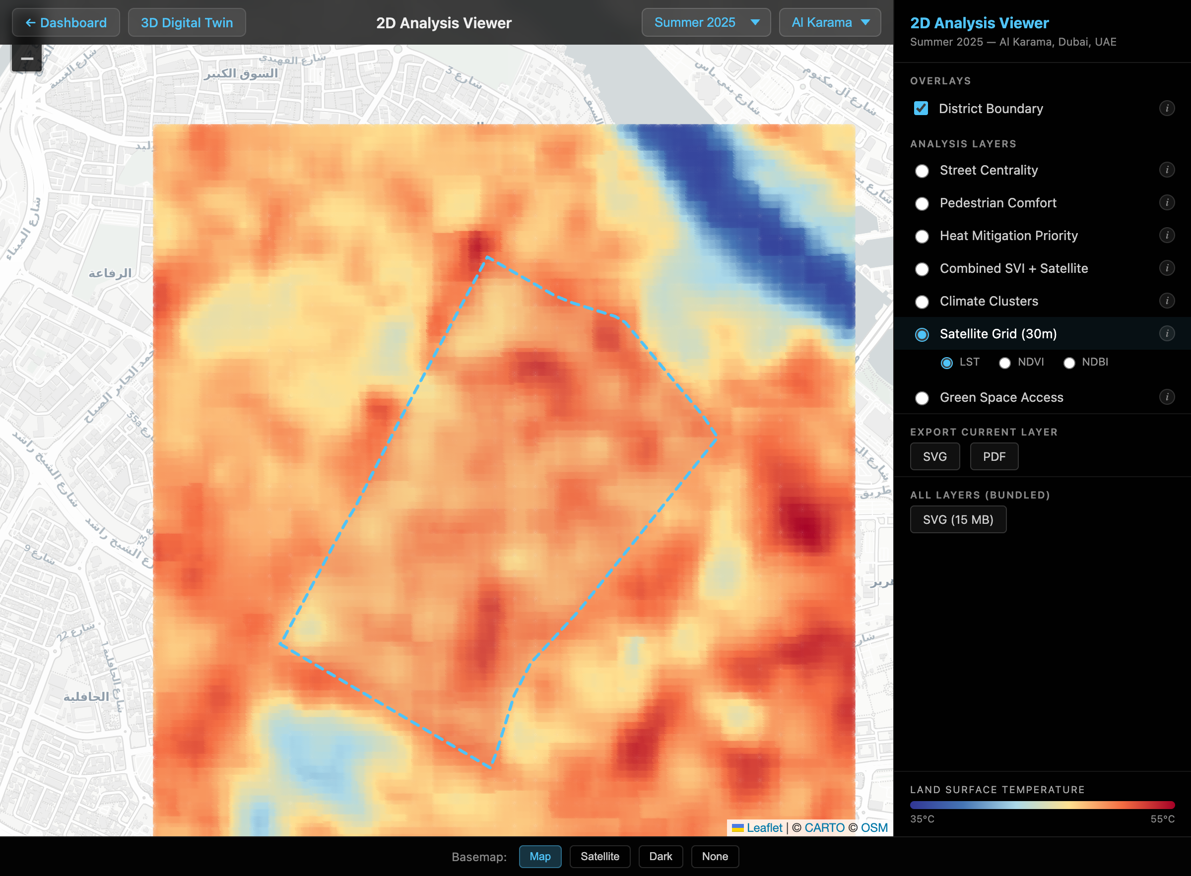
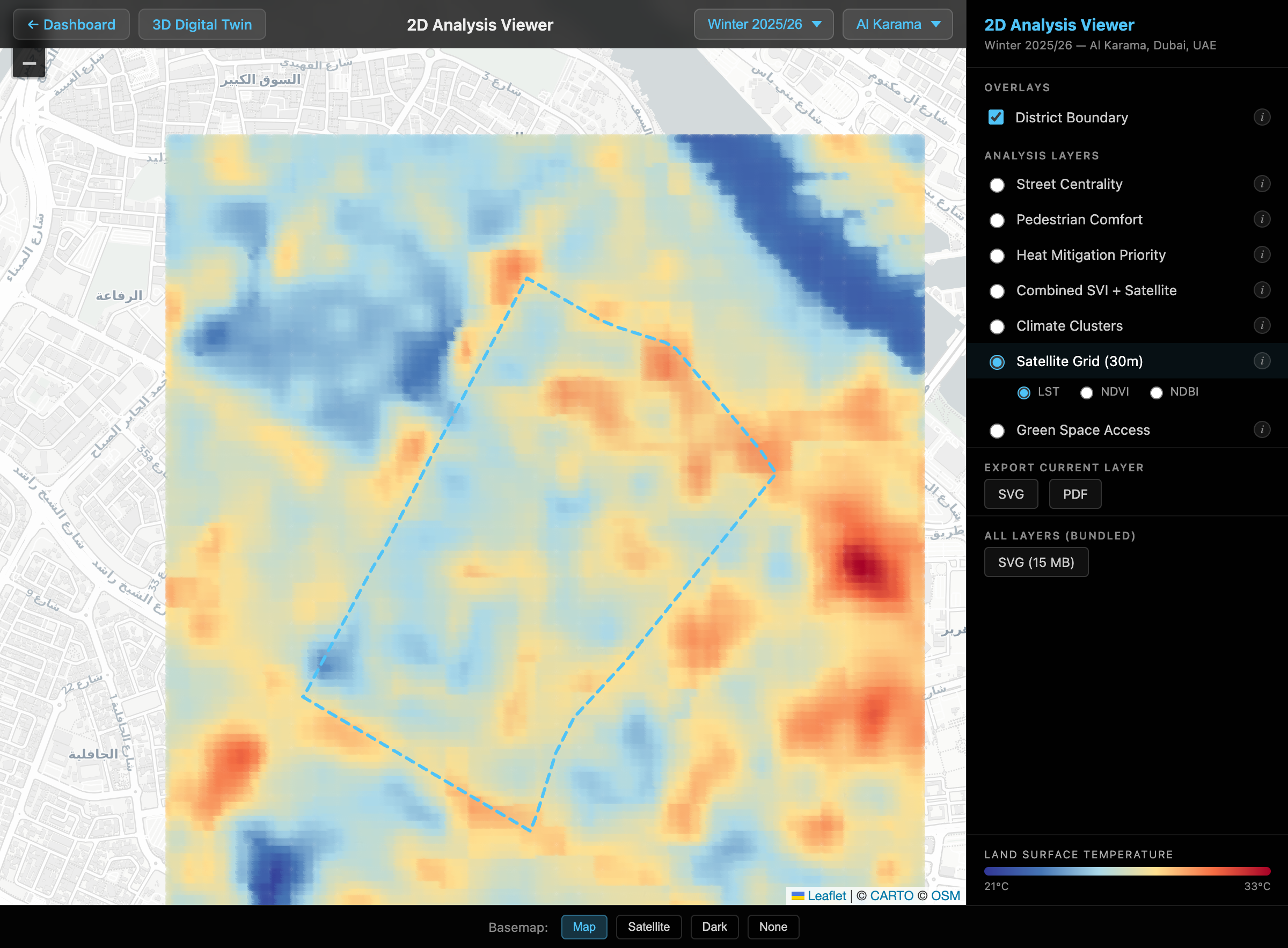
The Land Surface Temperature (LST) heatmaps below illustrate the seasonal contrast. Note that each map uses its own dynamic colour scale to highlight spatial variation within that season:
Summer 2025 — LST range 35–55°C. The district is dominated by red/orange, with hot-spots exceeding 54°C in dense built-up areas. Cooler blue patches correspond to parks and irrigated vegetation.Winter 2025/26 — LST range 21–33°C. The same district appears far cooler, with widespread blue tones. Relative hot-spots still align with dense impervious surfaces, but at 21°C lower than summer.
10.5 3D Viewer: Summer vs Winter
The 3D Digital Twin viewer reflects seasonal differences in real-time GPU sun shadows, pre-computed shadow overlays, and shade coverage charts. The screenshots below show the same noon south-facing view with GPU Sun Shadows and Building Shadows enabled:
Summer 2025 — Sun at 83.2° altitude. Shadows fall almost directly beneath buildings; rooftops and facades are uniformly lit.Winter 2025/26 — Sun at 43.2° altitude. Long shadows extend northward from buildings, creating shaded streets between blocks.
How to explore: Open the 3D Digital Twin and use the season dropdown in the top navigation bar. The time slider at the bottom animates the sun through the day — try comparing 8 AM shadows between seasons to see how winter's low sun creates long east-facing shadows.
10.7 Temporal Comparison: 2020 vs 2025
By adding Summer 2020 and Winter 2020/21 to the analysis, we can observe how Al Karama's urban microclimate has evolved over five years. The 2020 seasons use Landsat 8 and Sentinel-2 imagery (Landsat 9 was not available until late 2021); the pipeline merges available collections gracefully.
Summer: 2020 vs 2025
Metric
Summer 2020
Summer 2025
Change
LST mean
49.1°C
48.3°C
−0.8°C
LST max
55.4°C
54.8°C
−0.6°C
NDVI mean
0.082
0.096
+0.014
NDBI mean
0.028
0.033
+0.005
Winter: 2020/21 vs 2025/26
Metric
Winter 2020/21
Winter 2025/26
Change
LST mean
27.0°C
27.0°C
~0°C (unchanged)
LST max
31.9°C
33.0°C
+1.1°C
NDVI mean
0.103
0.114
+0.012
NDBI mean
0.017
0.010
−0.007
Key findings over 5 years:
Vegetation is the clearest signal. NDVI increased by +0.012 to +0.014 across both seasons, suggesting Al Karama has become slightly greener — consistent with Dubai's ongoing urban greening and landscaping programmes.
Summer LST dropped modestly (−0.8°C). This could reflect increased vegetation or shade, though year-to-year weather variability (a hotter satellite overpass day in 2020) cannot be ruled out from a single composite.
Winter LST is essentially unchanged at the mean level, though the peak hotspot temperature rose by ~1°C — possibly indicating localised new dense construction absorbing more heat.
NDBI trends are mixed — slightly higher in summer 2025 (+0.005) but lower in winter 2025 (−0.007). The differences are small and likely reflect spectral variability more than meaningful changes in built-up area.
Overall the changes are modest and within the range of year-to-year variability. The NDVI increase is the most consistent finding across both seasons.
Methodology notes
Building footprints: The same present-day OSM building data is used for shade analysis in both 2020 and 2025, so shade coverage differences reflect solar geometry only (negligible over 5 years), not changes in building stock. A future refinement could use historical footprints where available.
Satellite composites: Each season uses a median composite of all available cloud-free scenes in the date range (Summer 2020: 15 Landsat + 34 Sentinel-2; Winter 2020/21: 10 Landsat + 30 Sentinel-2). More scenes generally produce smoother composites.
Interactive Change Detection Map
In addition to comparing seasons via the dropdown, both viewers offer a dedicated 5-Year Change layer that computes and visualises pixel-by-pixel differences between Summer 2020 and Summer 2025. For each of the 90,300 grid points the layer displays:
ΔLST — temperature change on a blue (cooled) → white (no change) → red (warmed) diverging scale, clamped to ±3°C.
ΔNDVI — vegetation change on a brown (loss) → white → green (greened) scale, clamped to ±0.2.
ΔNDBI — built-up change on a blue (reduced) → white → orange-red (increased) scale, clamped to ±0.2.
Clicking any point shows both years' original values alongside the delta, making it easy to distinguish areas of genuine change from noise. The layer is season-independent (it always compares the same two summer composites) and persists when switching the season dropdown.
How to explore: Use the season dropdown in either the 3D Digital Twin or the 2D map viewer to switch between all four seasons. Compare the same metric (e.g., LST heatmap) across Summer 2020 vs Summer 2025 to isolate temporal changes from seasonal effects. Alternatively, enable the 5-Year Change layer for a direct pixel-by-pixel difference map with diverging colour scales.
10.6 Season-Independent Data
Some data layers do not change between seasons and are shared across both:
Building footprints and heights — structural, not seasonal
Tree canopy polygons — Dubai's irrigated urban trees are largely evergreen
Street network and centrality — infrastructure doesn't change
Street View GVI/SVF — Mapillary images are snapshots; we reuse the same values for both seasons
Points of Interest — from OpenStreetMap, not season-dependent
11. Key Findings
11.1 Correlations
Relationship
Correlation (r)
Interpretation
GVI ↔ NDVI
0.501
Street greenery matches satellite vegetation - data validates!
SVF ↔ LST
0.136
More sky exposure = slightly hotter
GVI ↔ LST
-0.039
More greenery = slightly cooler (weak)
NDVI ↔ LST
-0.040
Vegetation cools surfaces (weak)
Why are temperature correlations weak?
Satellite LST measures surface temperature, but pedestrians experience air temperature and radiant heat. Also, our measurements are at different times (satellite = specific overpass time, street view = whenever image was captured).
11.2 Main Takeaways
Al Karama is hot: Mean surface temperature of 48.3°C in summer
Very little vegetation: Only 3.55% green view, 0.096 NDVI
Most streets uncomfortable: 71% have low pedestrian comfort
Shade helps: Areas with low SVF are more comfortable
78% needs intervention: High or critical priority for heat mitigation
12. Limitations
1. Temporal mismatch: Street view images are from various dates, satellite data is from summer 2025 (Jun–Sep) and winter 2025/26 (Dec–Feb). Both Landsat and Sentinel-2 are filtered to matching seasonal windows, but street view images were captured at different times and are reused across seasons.
2. LST ≠ Air temperature: Satellite measures surface temperature, not what pedestrians feel. Actual thermal comfort depends on air temperature, humidity, wind, and radiant heat.
3. Resolution limits: Satellite data is 10-30m resolution. Fine-scale variations (individual trees, building shadows) are smoothed out.
4. Street view sampling bias: Mapillary images are crowdsourced, so coverage depends on where people drove/walked with cameras. Some areas may have gaps.
5. Two seasons only: We analyze summer (Jun–Sep) and winter (Dec–Feb). Transitional seasons (spring, autumn) are not covered. Additionally, winter satellite data may have fewer cloud-free scenes than summer in this region.
6. GHSL height classes are coarse: The GHSL Built-C dataset provides 5 height bands, not precise heights. Buildings are assigned midpoint values (e.g., all 6-15m buildings get 10.5m). This means 94% of buildings share one of only 5 possible height values. GHSL Built-H caps at ~40m, underestimating the tallest buildings in Al Karama.
13. Output Files Reference
Interactive Viewers
File
Description
index.html
Main dashboard with links to all visualizations
viewer.html
3D Digital Twin — buildings, shade, thermal, mobility, POIs (deck.gl, 13 layers)
Area manifest with seasons metadata, sun info, layer paths
—
buildings.geojson
Building footprints with GEE-enhanced heights
3,243
canopy.geojson
Tree canopy polygons with IDW-interpolated heights
1,033
streets.geojson
Street network with centrality, PCI, LST, priority
5,656
pois.json
Points of interest (8 categories, Overpass API)
1,290
street_metrics.json
Street-level aggregated metrics
5,656
segment_comfort.json
Pedestrian comfort by street segment
420
Season-specific files (under summer_2025/ and winter_2025/):
File
Description
Records
combined_svi.json
Street-level GVI/SVF + satellite LST/NDVI
10,098
satellite_grid.json
Satellite LST/NDVI/NDBI grid (30m, subsampled)
20,000
priority_points.json
Heat mitigation priority scores and levels
11,576
clusters.json
K-means climate cluster assignments
10,098
distance_to_green.json
Distance to nearest green space
11,576
street_shade.csv
Shade % per street per hour
5,656
shadows/shadows_HH.geojson
Shadow polygons per hour (×7 files)
—
Python Scripts
Script
Purpose
setup_gee.py
Test Google Earth Engine connection
satellite_analysis.py
Download and analyze satellite data (--season flag)
satellite_full_area.py
Full area grid analysis at 10m (--season flag)
thermal_sharpening.py
Downscale LST from 30m to 10m using NDVI regression (--season flag)
combined_analysis.py
Merge street-level GVI/SVF with satellite thermal data (--season flag)
heat_mitigation_priorities.py
Calculate intervention priorities
walking_route_analysis.py
Pedestrian comfort analysis
network_analysis_v3.py
Street network centrality
quick_analyses.py
Correlations, clusters, accessibility
gee_building_heights.py
Extract GHSL/nDSM building heights from GEE, merge with OSM
shade_analysis.py
Building + tree canopy shadow projection and street shade coverage analysis (--season flag)
seasons_config.py
Season definitions (dates, solar params) — shared config module
fetch_canopy_height.py
Fetch Meta 1m canopy height data from GEE, extract polygons, and assign heights via IDW interpolation
14. Field Survey Guide
14.1 Objective
Validate estimated building heights by conducting on-site measurements using clinometer-based distance-angle methods. A 50m-radius test area was selected around a central Mapillary camera location.
14.2 Test Area
Property
Value
Location
Al Karama, Dubai (25.2421°N, 55.3048°E)
Radius
50m
Camera positions
8 Mapillary camera locations within the test area
Center camera ID
827604215891753
14.3 Measurement Protocol
Buildings to measure:
Select 3–5 buildings for calibration
Vary heights: include low-rise, mid-rise, and high-rise
Note GPS coordinates for each building
Take reference photos
For each building:
Stand 20–50m away
Measure distance to base (GPS or tape measure)
Measure angle to rooftop (clinometer app)
Count floors as backup estimate
Take a photo with a person or car for scale reference
Building Height = Distance × tan(Angle) + Observer Height
14.4 Recommended Apps
Platform
Apps
iOS
Measure (built-in), Theodolite
Android
Smart Measure, Clinometer
Both
GPS Coordinates app
Tip: Measure buildings visible from the Mapillary camera positions. The center point (camera 827604215891753) is at 25.242071°N, 55.304779°E. Measurement points at the NE, NW, SE, and SW corners of the 50m radius provide good vantage points for surveying nearby buildings.
Tools & Libraries Used
Tool
Purpose
License
ZenSVI
Download Mapillary images, calculate GVI/SVF
Open source
Google Earth Engine
Access satellite imagery
Free for research
OSMnx
Download OpenStreetMap street networks
MIT
NetworkX
Graph/network analysis
BSD
scikit-learn
K-means clustering
BSD
GeoPandas
Geospatial data handling
BSD
Leaflet.js
Interactive web maps
BSD
deck.gl
3D WebGL map visualisation with GPU shadow rendering
MIT
SciPy
Spatial KD-tree for IDW canopy height interpolation
Monocular depth estimation uses a neural network to predict a per-pixel depth map from a single image. We tested DepthAnythingV2, a foundation model that produces a relative depth map where each pixel is assigned a value indicating its distance from the camera (blue = far, red = near).
The initial hypothesis was that depth maps from street-view images could be used to estimate building heights, supplementing or replacing satellite-derived height data.
A.2 What Was Done
26 test images from a 50m-radius area (centred on Mapillary camera 827604215891753) were processed as a proof-of-concept. The model successfully produced visually plausible depth maps distinguishing foreground elements (cars, people) from background structures (buildings, sky).
A.3 Why It Was Dropped
Fundamental limitation: relative depth only. Monocular depth estimation produces relative distances (pixel A is closer than pixel B), not absolute distances in metres. Without camera calibration parameters (focal length, sensor size) — which Mapillary images do not reliably provide — there is no way to convert the depth map into real-world measurements.
This means depth estimation cannot answer "this building is 25m tall" — only "this building is farther away than this car." Building heights require absolute measurements, which this technique cannot provide from the available data.
A.4 What Would Make It Viable
Requirement
What It Enables
Stereo image pairs (two images of the same scene from known positions)
Triangulation for absolute distance
Camera intrinsics (focal length, sensor size)
Metric depth from single images
LiDAR ground truth
Calibration of relative depth to absolute values
None of these were available from the Mapillary dataset. Adding more single-view images would not resolve the limitation — the problem is the absence of calibration data, not the quantity of images.
A.5 Alternative Used
Building heights were instead derived from satellite sources via Google Earth Engine (see Section 5), achieving 99.5% coverage across 3,243 buildings using GHSL Built-C, GHSL Built-H, nDSM (ALOS–SRTM), and OSM survey data.